Experiment #2: Truss Solver
E (GPa) |
σyield (MPa) |
A (m2)
Position (m) |
Force (kN)
Controls:
- Click on nodes to select
- Click and drag to move nodes
- With a node selected click on other nodes to toggle connection.
- Use the mouse wheel to rotate a fixed or roller node.
- To delete a node select it then click ‘Trash’
- Double-Click on a node to add force in the direction of the next mouse click.
- Use the Position and Force boxes to enter new values for the selected node.
Check out the developer console (F12) for the math.
About
One of the first real ‘engineering’ classes that we took at school was Statics. Statics in engineering is the study of the loads on systems that do not move (a=0). My initial goal for this project was to create a solver for the classic truss problem that you solve a million times.
The biggest difference between my goal and what I made comes from that fact that these elements do move when you solve the problem. That is because I found that the problem was just as easily solved as a 2d Finite Element Analysis (FEA) problem as it was a classic truss problem, and who doesnt like some good deflection. With some helpful online resources I managed to cobble together this little demo.
FEA Explained
A Finite Element Analysis is an analysis conducted on… a finite number of elements. Using some clever math we can arrange the problem into a linear algerbra problem which will allow us to solve it easily. The math looks like this. $$Ku=f$$ Where \(K\) is the global stiffness matrix, \(u\) is the displacement vector, and \(f\) is the force vector.
\(K\) is the trickiest part of this so we will talk about it first. Consider a single 2d structural element, which looks like this.  This element has 4 degrees of freedom (\(u_0\), \(v_0\), \(u_1\), \(v_1\)) and can only carry loads (\(F\)) along it’s axis. Hook’s Law for the force in a spring is \(f=kx\).
In our case: $$k = \frac{AE}{L}$$ Where: \(A\) is the cross-section area of the element, \(E\) is the Young’s Modulus of the element material and \(L\) is the element’s length.
And: $$x = (U_1cos(\theta) + V_1sin(\theta)) - (U_0cos(\theta) + V_0sin(\theta)) = \begin{bmatrix}-cos(\theta) & -sin(\theta) & cos(\theta) & sin(\theta)\end{bmatrix} \begin{bmatrix}u_0 \\ v_0 \\ u_1 \\ v_1\end{bmatrix}$$ All together: $$\begin{bmatrix}f_{x0} \\ f_{y0} \\ f_{x1} \\ f_{y1}\end{bmatrix} = \begin{bmatrix}-cos(\theta) \\ -sin(\theta) \\ cos(\theta) \\ sin(\theta)\end{bmatrix}F = \frac{AE}{L}\begin{bmatrix}-cos(\theta) & -sin(\theta) & cos(\theta) & sin(\theta)\end{bmatrix} \begin{bmatrix}u_0 \\ v_0 \\ u_1 \\ v_1\end{bmatrix}$$
Rearranged we get our local stiffness matrix: $$\begin{bmatrix}f_{x0} \\ f_{y0} \\ f_{x1} \\ f_{y1}\end{bmatrix} = \frac{AE}{L} \begin{bmatrix} cos^2(\theta) & cos(\theta)sin(\theta) & -cos^2(\theta) & -cos(\theta)sin(\theta) \\ cos(\theta)sin(\theta) & sin^2(\theta) & -cos(\theta)sin(\theta) & sin^2(\theta) \\ -cos^2(\theta) & -cos(\theta)sin(\theta) & cos^2(\theta) & cos(\theta)sin(\theta) \\ -cos(\theta)sin(\theta) & -sin^2(\theta) & cos(\theta)sin(\theta) & -sin^2(\theta) \end{bmatrix} \begin{bmatrix}u_0 \\ v_0 \\ u_1 \\ v_1\end{bmatrix}$$
After obtaining the local stiffness matrix for each element we can then assemble the global stiffness matrix and the corresponding force and displacement vectors. To do so we must slot the local entries into the correct location in the global matrix. We will use the following truss as an example: 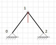
With the local stiffness matricies \(k^{01}\) and \(k^{12}\). We can create \(K\) as follows. $$K = \begin{bmatrix} k^{01}_{1, 1} & k^{01}_{1, 2} & k^{01}_{1, 3} & k^{01}_{1,4} & 0 & 0 \\ k^{01}_{2, 1} & k^{01}_{2, 2} & k^{01}_{2, 3} & k^{01}_{2,4} & 0 & 0 \\ k^{01}_{3, 1} & k^{01}_{3, 2} & k^{01}_{3, 3} + k^{12}_{1, 1} & k^{01}_{3,4} + k^{12}_{1, 2} & k^{12}_{1, 3} & k^{12}_{1, 4} \\ k^{01}_{4, 1} & k^{01}_{4, 2} & k^{01}_{4, 3} + k^{12}_{2, 1} & k^{01}_{4,4} + k^{12}_{2, 2} & k^{12}_{2, 3} & k^{12}_{2, 4} \\ 0 & 0 & k^{12}_{3, 1} & k^{12}_{3, 2} & k^{12}_{3, 3} & k^{12}_{3, 4} \\ 0 & 0 & k^{12}_{4, 1} & k^{12}_{4, 2} & k^{12}_{4, 3} & k^{12}_{4, 4} \end{bmatrix}$$
Substituting into our original equation \(Ku=f\) we get this: $$\begin{bmatrix} k^{01}_{1, 1} & k^{01}_{1, 2} & k^{01}_{1, 3} & k^{01}_{1,4} & 0 & 0 \\ k^{01}_{2, 1} & k^{01}_{2, 2} & k^{01}_{2, 3} & k^{01}_{2,4} & 0 & 0 \\ k^{01}_{3, 1} & k^{01}_{3, 2} & k^{01}_{3, 3} + k^{12}_{1, 1} & k^{01}_{3,4} + k^{12}_{1, 2} & k^{12}_{1, 3} & k^{12}_{1, 4} \\ k^{01}_{4, 1} & k^{01}_{4, 2} & k^{01}_{4, 3} + k^{12}_{2, 1} & k^{01}_{4,4} + k^{12}_{2, 2} & k^{12}_{2, 3} & k^{12}_{2, 4} \\ 0 & 0 & k^{12}_{3, 1} & k^{12}_{3, 2} & k^{12}_{3, 3} & k^{12}_{3, 4} \\ 0 & 0 & k^{12}_{4, 1} & k^{12}_{4, 2} & k^{12}_{4, 3} & k^{12}_{4, 4} \end{bmatrix} \begin{bmatrix} u_0 \\ v_0 \\ u_1 \\ v_1 \\ u_2 \\ v_2 \end{bmatrix} = \begin{bmatrix} f_{x0} \\ f_{y0} \\ f_{x1} \\ f_{y1} \\ f_{x2} \\ f_{y2} \end{bmatrix} $$
The final trick to solving this equation is to eliminate rows and columns for nodes that are fixed. In this example we can remove the rows and columns corresponding to the nodes \(0\) and \(2\) or indexes \(0\), \(1\), \(5\) and \(6\). Considering that the displayed force is only in the y direction our final problem looks like this: $$\begin{bmatrix} k^{01}_{3, 3} + k^{12}_{1, 1} & k^{01}_{3,4} + k^{12}_{1, 2} \\ k^{01}_{4, 3} + k^{12}_{2, 1} & k^{01}_{4,4} + k^{12}_{2, 2}\\ \end{bmatrix} \begin{bmatrix} u_1 \\ v_1 \end{bmatrix} = \begin{bmatrix} 0 \\ f_{y1} \end{bmatrix} $$
After solving for \(u_1\) and \(v_1\) we can substitute the values we get back into the full problem above and matrix multiply to get the reaction forces.